2.4 Post-processing With Stacked X-ray Spectrum
Several ways post-processing:
1. Determine Usable Energy Range
Before fitting, check:
source-contribution fraction per energy bin,
net-count fraction after background subtraction.
Use Xstack.visual.view.valid_energy_range_plot to identify an analysis interval where completeness and net-count quality are acceptable:
from Xstack.view.visual import valid_energy_range_plot
from matplotlib import pyplot as plt

#--- specify the file names...
# src_name = ...  	# source spectrum file
# grp_name = ...	# grouped source spectrum file to be created
# bkg_name = ...  	# background spectrum file
# arf_name = ...  	# ARF file
# rmf_name = ...  	# RMF file
# fene_name = ...  	# file storing the energy range of the source spectrum

fig, ax1 = plt.subplots(figsize=(4,4))
valid_energy_range_plot(fene_name,src_name,grp_name,bkg_name,rmf_name,ax=ax1)

ax1.set_xscale("log")
ax1.set_xlim(0.2,10)
x_ticks = [0.2, 0.4, 1.0, 2.3, 4.0, 8.0]
ax1.set_xticks(x_ticks)
ax1.set_xticklabels([str(x) for x in x_ticks])
Output shown in Fig. 3.
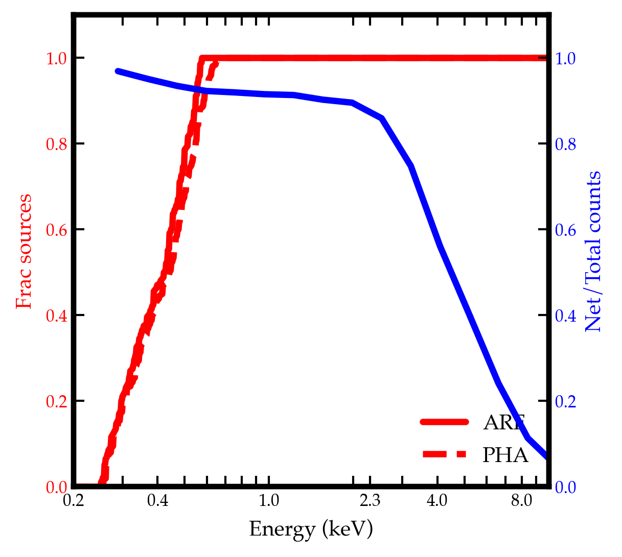
Fig. 3 Valid energy range plot.
2. Visualize Stacked Spectral Shape
Generate a quick data/ARF diagnostic curve:
Xstack.visual.view.make_dataarf_plot
This is useful for rapid sanity checks of overall shape (for example, power-law-like trends, soft excess, or hard curvature).
from Xstack.view.visual import make_dataarf_plot
from Xstack.utils.pi import make_grpflg
from matplotlib import pyplot as plt

#--- specify the file names...
# src_name = ...  	# source spectrum file
# grp_name = ...	# grouped source spectrum file to be created
# bkg_name = ...  	# background spectrum file
# arf_name = ...  	# ARF file
# rmf_name = ...  	# RMF file
# fene_name = ...  	# file storing the energy range of the source spectrum

# create a grouped PI spectrum
with fits.open(rmf_name) as hdu:
    ebo = hdu["EBOUNDS"].data
ene_lo = ebo["E_MIN"]
ene_hi = ebo["E_MAX"]
ene_ce = (ene_lo + ene_hi) / 2
eene = np.logspace(np.log10(0.2),np.log10(ene_ce.max()),18)
eelo = eene[:-1]
eehi = eene[1:]
make_grpflg(
    src_name,   # source spectrum file
    grp_name,   # output grouped spectrum file
    method='EDGE',  # grouping spectrum by fixed edges, as specified in `eelo` and `eehi`
    rmf_fname=rmf_name,  # RMF file to be used for reading PI energy channels
    eelo=eelo,  # lower edges of the grouped energy channels
    eehi=eehi   # upper edges of the grouped energy channels
)

# make data/arf plot
fig, ax1 = plt.subplots(figsize=(4,4))
# for the grouped spectrum
make_dataarf_plot(
    src_name,
    bkg_name,
    arf_name,
    rmf_name,
    grp_name,
    normalize_at=4,	# normalize at 4 keV
    plot=True,
    ax=ax1,
    fmt="o-",ms=3.5,lw=0.20,c="k",capsize=0.,elinewidth=1.0,mec="k",mfc="#f9d7a7",alpha=0.8,zorder=1,label="binned spec"	# plotting kwargs
) # this plots EF(E), or equivalently leed in xspec; a powerlaw with photon index of 2 should look flat in this plot
# for the ungrouped spectrum
make_dataarf_plot(
    src_name,
    bkg_name,
    arf_name,
    rmf_name,
    normalize_at=4,	# normalize at 4 keV
    plot=True,
    ax=ax1,
    fmt="o",ms=0.3,lw=0.1,c="gray",alpha=0.5,zorder=-5,label="unbinned spec"
)
Output shown in Fig. 4.
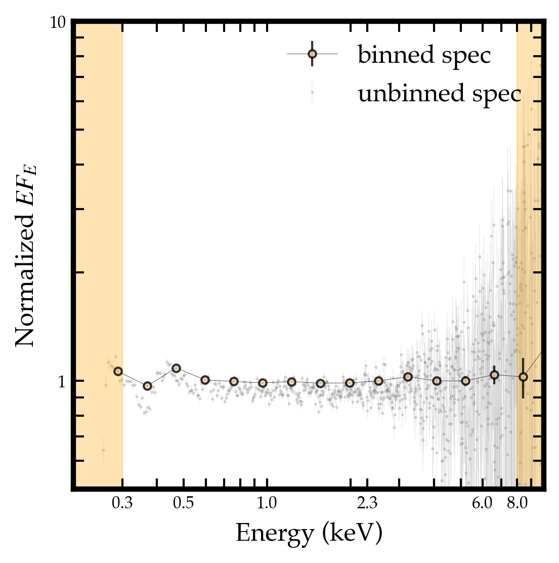
Fig. 4 Data/arf plot.
3. Response Inspection
Inspect RMF behavior if needed:
Xstack.visual.view.view_rmf
This helps diagnose dispersion broadening and response-smearing effects after rest-frame shifting + stacking. Or simply check any individual RMF.
from Xstack.visual.view import view_rmf
from matplotlib import pyplot as plt

fig, (ax1, ax2, ax3) = plt.subplots(1, 3, figsize=(18, 5))
cmap = Colormap("cmasher:eclipse").to_mpl()
color_inst = Colormap("cmasher:eclipse")(0.4).hex
color_res = Colormap("cmasher:eclipse")(0.7).hex

#--- ax1: xmm-pn
pn_rmf_fname = f"./responses/pn-med-5.rmf"
_, im, cbar = view_rmf(pn_rmf_fname,fig=fig,ax=ax1,log_scale=True,cmap=cmap,)
ax1.text(
    0.7,0.25,r"$R@2\mathrm{keV}\sim15$",transform=ax1.transAxes,ha="center",va="center",
    fontsize=24,color=color_res,path_effects=[pe.Stroke(linewidth=1.5,foreground=color_res),pe.Normal()]
)
ax1.text(
    0.05,0.85,r"XMM/PN",transform=ax1.transAxes,ha="left",va="bottom",color=color_inst,
    fontsize=20,path_effects=[pe.Stroke(linewidth=1.5,foreground=color_inst),pe.Normal()],
    bbox=dict(boxstyle="round,pad=0.3",facecolor="gray",edgecolor="none",alpha=0.8),
)

im.set_clim(1e-6,0.5)
cbar.update_normal(im)
ticks = np.logspace(np.log10(1e-6),np.log10(0.5),4)
cbar.set_ticks(ticks)
cbar.set_ticklabels([f"{t:.0e}" for t in ticks])
ax1.set_xlim(0,16)
ax1.set_xlabel("Output channel energy (keV)", fontsize=18)
ax1.set_ylim(0,16)
ax1.set_ylabel("Input photon energy (keV)", fontsize=18)


#--- ax2: xmm-rgs
rgs_rmf_fname = f"./responses/RGS_R1O1.rmf"
_, im, cbar = view_rmf(rgs_rmf_fname,fig=fig,ax=ax2,log_scale=True,cmap=cmap,)
ax2.text(
    0.7,0.25,r"$R@2\mathrm{keV}\sim200$",transform=ax2.transAxes,ha="center",va="center",
    fontsize=24,color=color_res,path_effects=[pe.Stroke(linewidth=1.5,foreground=color_res),pe.Normal()]
)
ax2.text(
    0.05,0.85,r"XMM/RGS",transform=ax2.transAxes,ha="left",va="bottom",color=color_inst,
    fontsize=20,path_effects=[pe.Stroke(linewidth=1.5,foreground=color_inst),pe.Normal()],
    bbox=dict(boxstyle="round,pad=0.3",facecolor="gray",edgecolor="none",alpha=0.8),
)

im.set_clim(1e-6,0.5)
cbar.update_normal(im)
ticks = np.logspace(np.log10(1e-6),np.log10(0.5),4)
cbar.set_ticks(ticks)
cbar.set_ticklabels([f"{t:.0e}" for t in ticks])
ax2.set_xlim(0.3,2.4)
ax2.set_xlabel("Output channel energy (keV)", fontsize=18)
ax2.set_ylim(0.3,2.4)
ax2.set_ylabel("Input photon energy (keV)", fontsize=18)


#--- ax3: xrism-resolve
resolve_rmf_fname = f"./responses/resolve.rmf"
_, im, cbar = view_rmf(resolve_rmf_fname,fig=fig,ax=ax3,log_scale=True,cmap=cmap,)
ax3.text(
    0.7,0.25,r"$R@2\mathrm{keV}\sim400$",transform=ax3.transAxes,ha="center",va="center",
    fontsize=24,color=color_res,path_effects=[pe.Stroke(linewidth=1.5,foreground=color_res),pe.Normal()]
)
ax3.text(
    0.05,0.85,r"XRISM/Resolve",transform=ax3.transAxes,ha="left",va="bottom",color=color_inst,
    fontsize=20,path_effects=[pe.Stroke(linewidth=1.5,foreground=color_inst),pe.Normal()],
    bbox=dict(boxstyle="round,pad=0.3",facecolor="gray",edgecolor="none",alpha=0.8),
)

im.set_clim(1e-6,0.5)
cbar.update_normal(im)
ticks = np.logspace(np.log10(1e-6),np.log10(0.5),4)
cbar.set_ticks(ticks)
cbar.set_ticklabels([f"{t:.0e}" for t in ticks])
ax3.set_xlim(0,10)
ax3.set_xlabel("Output channel energy (keV)", fontsize=18)
ax3.set_ylim(0,10)
ax3.set_ylabel("Input photon energy (keV)", fontsize=18)
Output shown in Fig. 5.
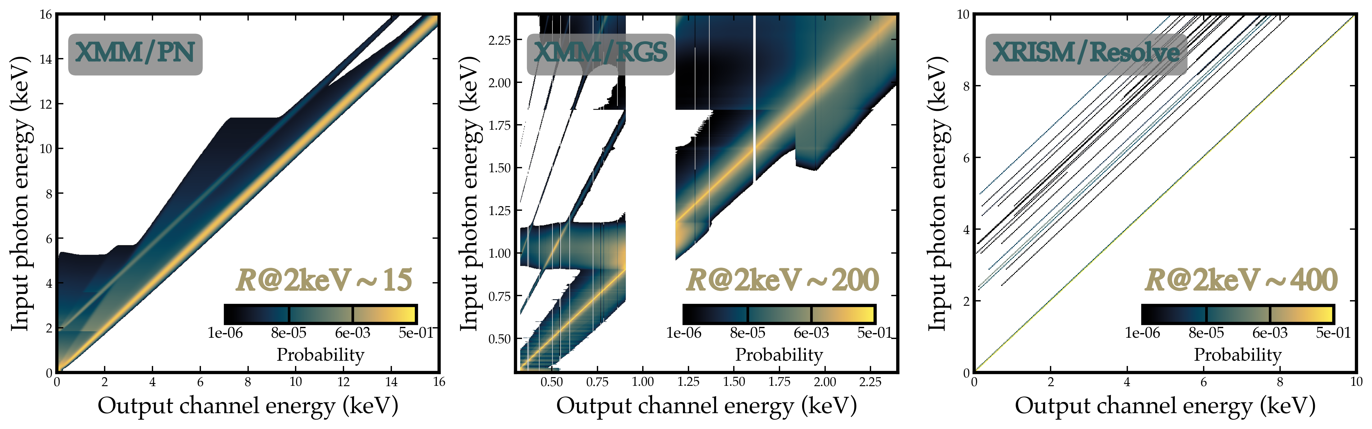
Fig. 5 RMF visualization.
4. Spectral Fitting (XSPEC)
With stacked PI spectrum, stacked background PI spectrum, ARF, and RMF generated by Xstack, proceed as with standard OGIP-style fitting workflows.
Recommended: PG-stat when source is Poisson-like and background handling is Gaussian-approximated.
5. Practical Notes
Xstack prioritizes preserving average spectral shape.
Absolute normalization should be interpreted with care in stacked products.
Keep track of
rsp_weight_method,int_rng, and source-selection choices when reporting fitted results.For
SHP, report the integration band (flux_energy_lo,flux_energy_hi/int_rng) andrsp_proj_gammafor reproducibility.